Forecasting the Energy Demand of Planned Production Lines

Before a company builds a production line it needs to know roughly how much electricity the line will use: for the operating budget, the grid connection and the size of the electrical installation. In practice that number is usually the rated power of each machine times a utilisation someone guessed.

The problem is that consumption isn't a property of the machine type. Two milling machines can differ a lot in base load, spindle, axis drives, cooling and pumps, and the same machine draws very different power while it warms up, waits, moves its axes, changes tools or cuts. So the working hypothesis of the thesis is: the structure of the model can be general, the parameters can't. The questions that follow are how far one structure carries across machine families, what a planner needs to know at which stage, and how wrong the forecast gets when that knowledge is missing.

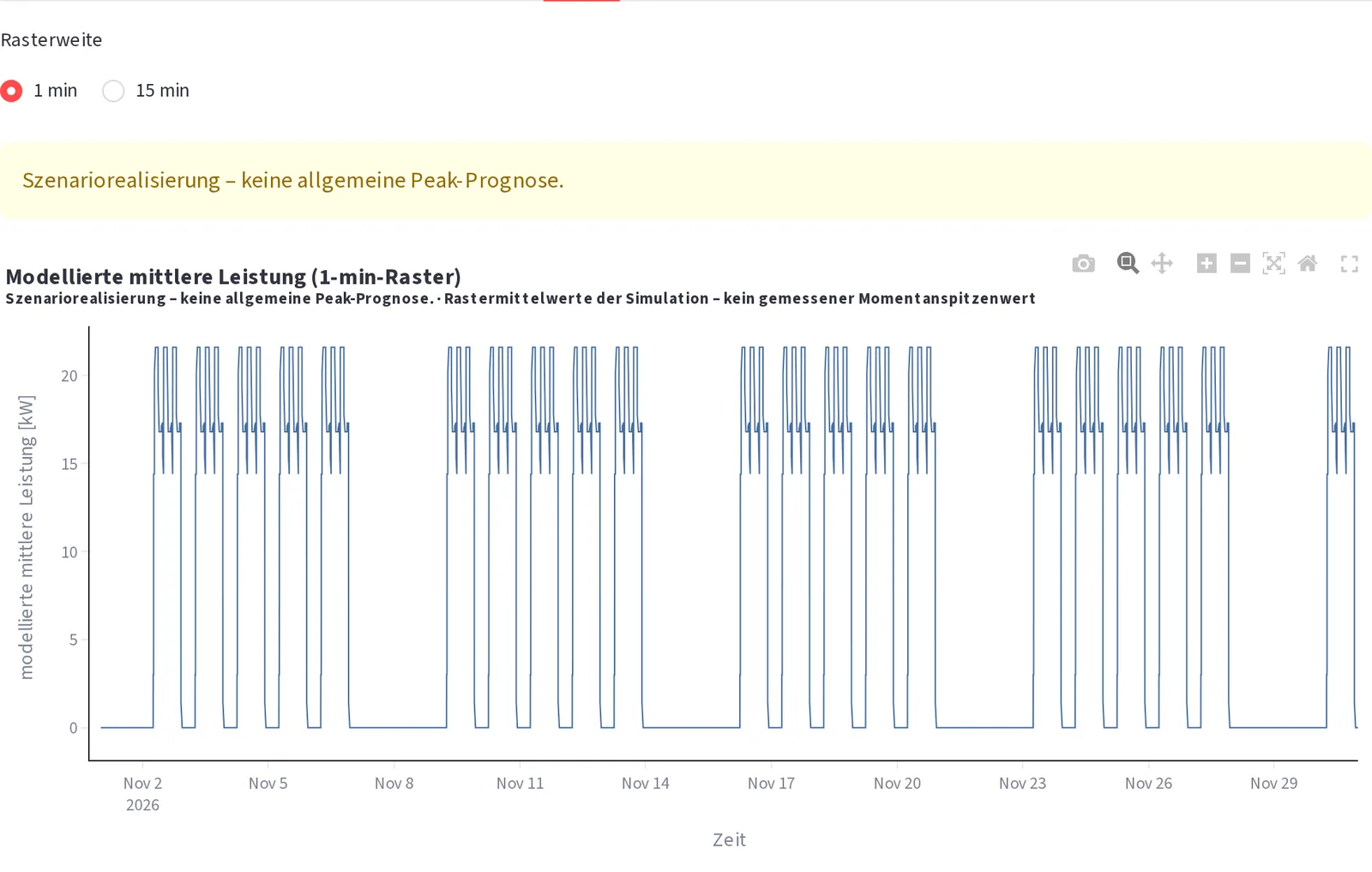
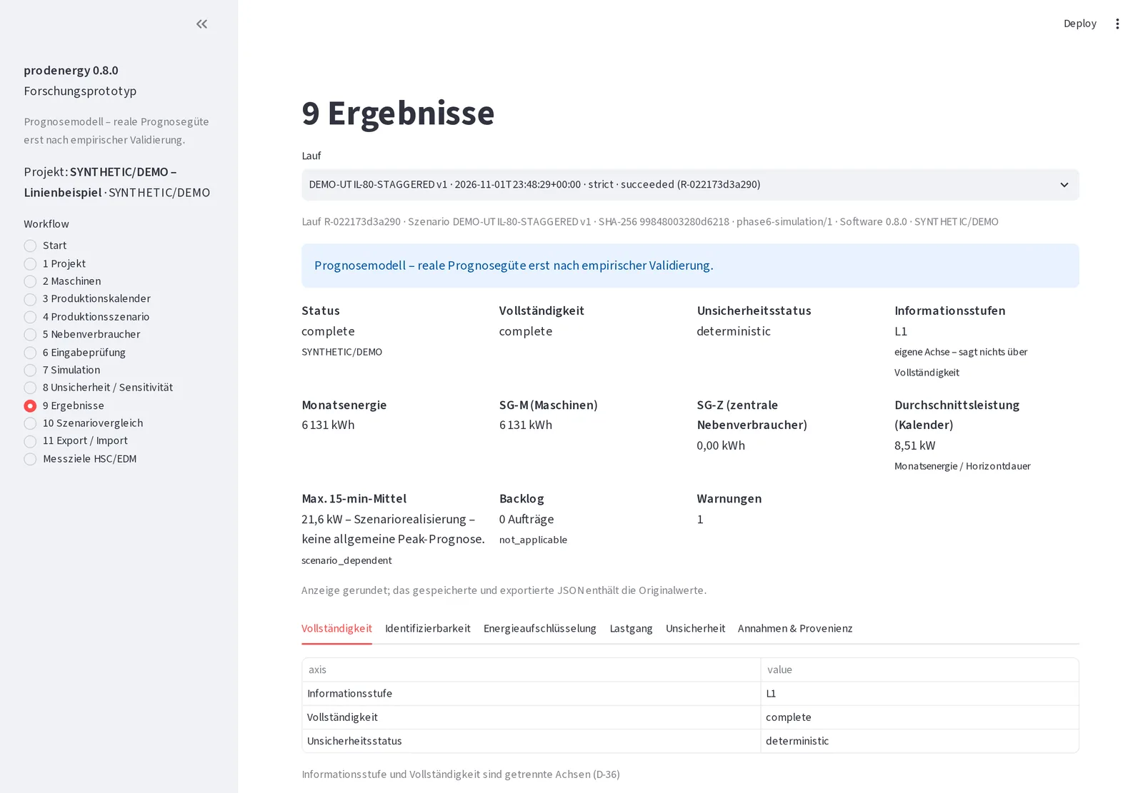
The software is called prodenergy. It runs a production simulation (which machine does what, when, in which state) and asks a machine model what each of those states costs. The output is a monthly energy balance and a load profile in 1- and 15-minute steps, with uncertainty ranges, a sensitivity analysis and a statement of how complete the result is.

• No silent defaults. If a parameter is missing, the result is unknown or incomplete. The software never fills in a typical value or a median from the literature.
• Every number has a source. Each parameter records where it comes from (a machine in the literature, manufacturer data, an assumption, a measurement) and at which level of knowledge: L1 structure and assumptions, L2 manufacturer data, L3 a measured machine.
• Nothing is counted twice. A measured base load already contains some auxiliary consumers. Those can't be added on top again.
• Runs are reproducible. Each run is tied to a versioned scenario schema, a hash of the scenario and hashes of the machine profiles it used.
• New machine families don't touch the core. Adding laser cutting shouldn't mean editing the scheduler.
• Peaks are labelled for what they are. At the planning stage a peak is one possible realisation of a scenario, not a peak forecast, and the UI and exports say that.

The most important decision was to keep the production flow and the energy physics apart. The simulator only knows states and durations. The machine packages only know what a state costs. Architecture tests hold that line: the simulator imports no machine package, machine packages never import each other, and the UI only talks to the application layer.

It's Python 3.11 with very few dependencies in the numerical core: dataclasses, enums and JSON schemas, with SQLite through SQLAlchemy for the workspace and Streamlit with Plotly for a local UI. All arithmetic is interval arithmetic on plain dataclasses, which means every intermediate value can be printed in a calculation trace when someone asks where a number came from. The literature database is JSON and TSV, built and checked by scripts, and the BibTeX for the manuscript is generated from it.

1. 1.

   Machine models

   Each machine family has its own set of states, profile format and calculator. A milling machine's power is built up per state: ready power, spindle power as a piecewise-linear or tabulated function of speed, a quadratic feed term per axis, a coolant term that can be switched off, and a cutting term. Inputs outside the measured range raise an error unless extrapolation is explicitly allowed.

2. 2.

   Scenario and calendar

   A scenario (production-scenario/1) sets the time horizon, shift windows, machine instances and shift policies, and exactly one of two modes: order-driven (orders, routings, operations) or utilisation-driven (time share per state).

3. 3.

   Scheduler

   Operations turn into state records on a gap-free timeline per machine. Setup happens once per operation, cycles once per part, and nothing is split across a shift or horizon boundary. The scheduler is deterministic, so the same scenario gives the same timeline every time.

4. 4.

   Energy

   Each segment asks its machine adapter for energy (energy_model_for(profile).compute_energy(...), cached per profile, state, duration and parameters). Central systems such as compressed air are calculated from when they're needed and booked to their own system boundary.

5. 5.

   Load profile

   Segment powers are rasterised to 1- and 15-minute means from the exact overlap with each interval, so no energy is lost or gained. The result lists energy per system boundary, a breakdown, the order backlog, how complete it is, and the full provenance.

Inclusion instead of guesswork. A measured ready power is an aggregate, and it declares which components it already contains. An extra component can only be added if it's provably not in there: either the list is declared complete, or the component is explicitly excluded. Otherwise the calculator raises DoubleCountingError or AmbiguousInclusionError rather than return a number that might be wrong.

Ranges, not point values. Parameters can be intervals, and the intervals carry through every sum and product. An unknown input makes everything that depends on it unknown. Completeness and level of knowledge are tracked separately: a measured machine (L3) is still incomplete if one of the states the scenario needs was never measured.

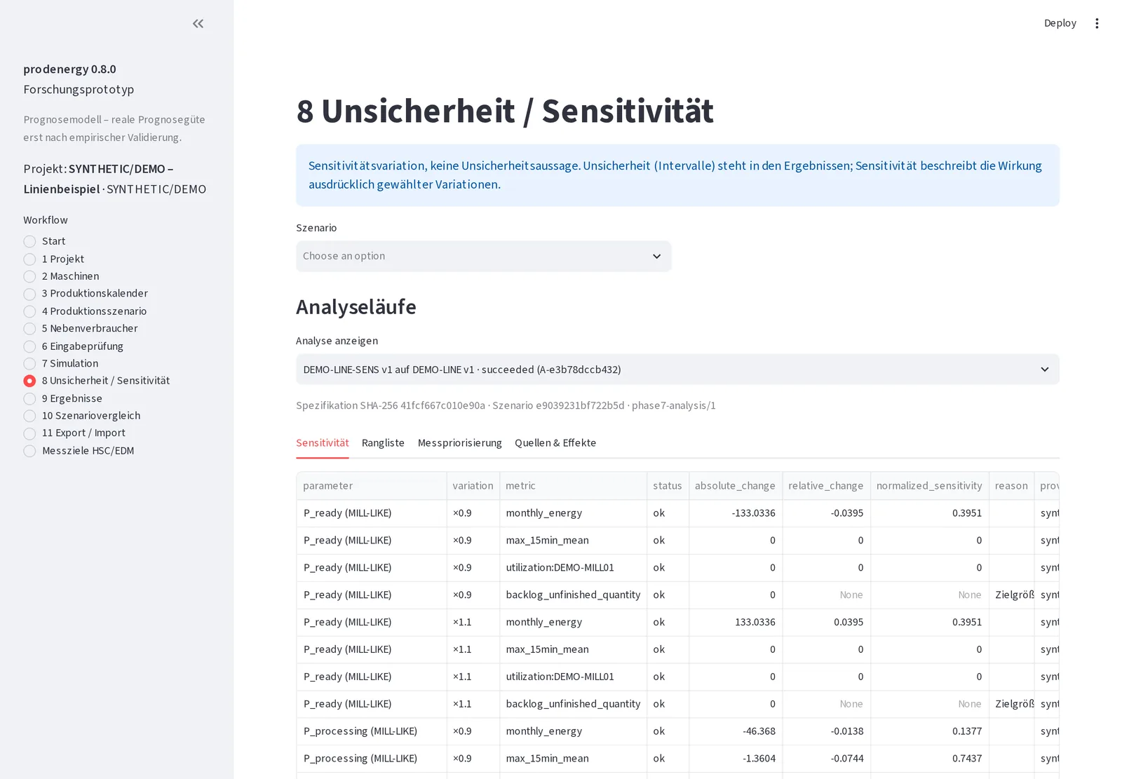
Knowing what to measure next. One-at-a-time variations along explicit parameter paths give normalised sensitivities and a ranking. An identifiability check then asks whether a parameter could be determined from the planned measurements at all. Together they say which measurement is worth the most.

• The published data doesn't line up. Measurements in papers use different system boundaries and rarely say what a base load includes. The literature base has 133 screened sources and 30 independent data lineages, and a parameter only counts as supported once there are at least three comparable measurement campaigns behind it.
• Six machine families, one scheduler. Spindles, EDM generators, laser sources, hydraulics and grinding wheels all have different states, and they all had to plug into a scheduler that knows none of them.
• Refactoring without moving a single number. When EDM was added, the shared model kernel was pulled out of the milling package. The milling profiles were regenerated byte for byte and the example outputs didn't change.
• Making `unknown` work everywhere. In arithmetic, results, UI and exports. It's more work than computing a number, but it's the whole point of the model.

Phases 1 to 8.5 of 10 are done: literature base, machine models, simulation, analysis, application and UI, and a draft of the manuscript. What works today is the whole chain from machine profiles to a monthly energy balance and load profile, with uncertainty and sensitivity analysis, scenario comparison, reproducible export bundles and a local UI with a synthetic demo project.

Tests

440, all passing

Machine families

Milling, sinker EDM, turning, laser cutting, grinding, presses

Literature base

133 screened sources, 39 source machines, 110 source measurements

Manuscript

Chapters 1 to 11 drafted, results chapters pending

After phase 10 (evaluation and the final manuscript), the obvious extensions are random process times, measured distributions instead of intervals, and a multi-user web interface.